how to draw realistic 3d plot in 2d

iii. Plotting

Producing plots and graphics is a very common chore for analysing data and creating reports. Scilab offers many ways to create and customize various types of plots and charts. In this section, nosotros present how to create 2d plots and contour plots. Then we customize the title and the fable of our graphics. We finally export the plots so that we can employ information technology in a study.

3.1 Overview

Scilab tin produce many types of 2d and 3D plots. It can create ten-y plots with the plot function, contour plots with the contour function, 3D plots with the surf function, histograms with the histplot role and many other types of plots. The most commonly used plot functions are presented in figure nineteen.

plot	2D plot
surf	3D plot
contour	contour plot
pie	pie chart
histplot	histogram
bar	bar chart
barh	horizontal bar chart
hist3d	3D histogram
polarplot	plot polar coordinates
Matplop	2D plot of a matrix using colors
Sgrayplot	smooth 2D plot of surface using colors
grayplot	2d plot of a surface using colors

Figure 19: Scilab plot functions

In society to get an instance of a 3D plot, we can but type the statement surf() in the Scilab console.

-->surf()
During the creation of a plot, nosotros use several functions in order to create the data or to configure the plot. The functions presented in figure 20 will be used in the examples of this section.

linspace	linearly spaced vector
feval	evaluates a function on a grid
legend	configure the fable of the current plot
title	configure the championship of the current plot
xtitle	configure the title and the legends of the current plot

Figure 20: Scilab functions used when creating a plot.

3.ii second plot

In this section, we nowadays how to produce a uncomplicated x-y plot. We emphasize the use of vectorized functions, which produce matrices of data in 1 function telephone call.

Nosotros begin past defining the role which is to be plotted. The myquadratic part squares the input statement x with the "ˆ"operator.

function f = myquadratic ( x )
f = x^2
endfunction
We can use the linspace role in guild to produce 50 values in the interval [1,x].

xdata = linspace ( i , x , l );
The xdata variable now contains a row vector with 50 entries, where the first value is equal to 1 and the last value is equal to 10. Nosotros tin can pass information technology to the myquadratic function and get the function value at the given points.

ydata = myquadratic ( xdata );
This produces the row vector ydata, which contains 50 entries. We finally employ the plot function so that the data is displayed equally an ten-y plot.

plot ( xdata , ydata )
Figure 21 presents the associated ten-y plot.

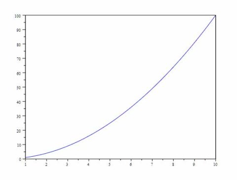
Effigy 21: A elementary ten-y plot.

Detect that we could accept produced the same plot without generating the intermediate assortment ydata. Indeed, the second input argument of the plot function tin be a part, as in the following session.

plot ( xdata , myquadratic )
When the number of points to manage is large, using functions directly saves significant amount of memory infinite, since it avoids generating the intermediate vector ydata.

iii.iii Profile plots

In this section, nosotros present the contour plots of a multivariate function and brand utilize of the contour function. This blazon of graphic is ofttimes used in the context of numerical optimization considering information technology draws functions of two variables in a mode that shows the location of the optimum.

The Scilab function contour plots contours of a function f. The contour function has the following syntax

contour(x,y,z,nz)
where

• x (resp. y) is a row vector of 10 (resp. y) values with size n1 (resp. n2),

• z is a real matrix of size (n1,n2), containing the values of the office or a Scilab function which defines the surface z=f(x,y),

• nz the level values or the number of levels.

In the following Scilab session, we use a elementary form of the contour function, where the function myquadratic is passed as an input statement. The myquadratic office takes two input arguments x1 and x2 and returns f(x1,x2) = x1^2 + x2^ii. The linspace function is used to generate vectors of data so that the function is analyzed in the range [−one,1]^2.

part f = myquadratic2arg ( x1 , x2 )
f = x1**2 + x2**ii;
endfunction
xdata = linspace ( -1 , ane , 100 );
ydata = linspace ( -ane , 1 , 100 );
contour ( xdata , ydata , myquadratic2arg , 10)
This produces the contour plot presented in figure 22.

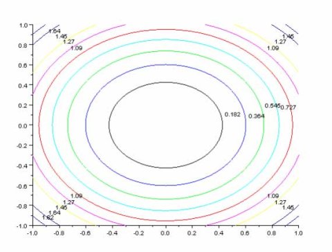
Effigy 22: Contour plot of the function f(x1,x2) = x1^2 + x2^two.

In exercise, it may happen that our function has the header z = myfunction ( x ), where the input variable ten is a row vector. The problem is that in that location is only one single input argument, instead of the two arguments required by the contour function. There are ii possibilities to solve this little problem:

 • provide the data to the contour office by making two nested loops,

• provide the data to the contour function by using feval,

• define a new function which calls the first one.

These 3 solutions are presented in this section. The first goal is to let the reader choose the method which best fits the state of affairs. The second goal is to prove that performances bug can be avoided if a consequent apply of the functions provided by Scilab is done.

In the following Scilab naive session, we define the part myquadratic1arg, which takes one vector as its unmarried input argument. And so we perform 2 nested loops to compute the zdata matrix, which contains the z values. The z values are computed for all the combinations of points (x(i),y(j)) ∈ R^2, for i = ane,2,…,nx and j = 1,2,…,ny, where nx and ny are the number of points in the x and y coordinates. In the end, we call the contour function, with the listing of required levels (instead of the previous number of levels). This gets exactly the levels nosotros want, instead of letting Scilab compute the levels automatically.

role f = myquadratic1arg ( x )
f = 10(one)**two + x(2)**2;
endfunction
xdata = linspace ( -i , i , 100 );
ydata = linspace ( -1 , 1 , 100 );
// Caution ! Two nested loops , this is bad.
for i = ane:length(xdata)
for j = i:length(ydata)
10 = [xdata(i) ydata(j)].';
zdata ( i , j ) = myquadratic1arg ( x );
terminate
finish
contour ( xdata , ydata , zdata , [0.1 0.3 0.5 0.vii])
The contour plot is presented in figure 23.

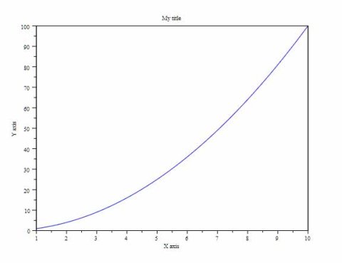
Figure 23: Profile plot of the function f(x1,x2) = x1^2+x2^ii – The levels are explicitly configured.

The previous script works perfectly. Still, it is non efficient considering it uses two nested loops and this should exist avoided in Scilab for performance reasons. Some other outcome is that we had to shop the zdata matrix, which might consume a lot of retention space when the number of points is large. This method should be avoided since it is a bad employ of the features provided past Scilab.

In the post-obit script, we use the feval function, which evaluates a function on a grid of values and returns the computed data. The generated grid is made of all the combinations of points (x(i),y(j)) ∈ R^2. We assume here that there is no possibility to change the function myquadratic1arg, which takes one input statement. Therefore, we create an intermediate function myquadratic3, which takes 2 input arguments. Once done, nosotros laissez passer the myquadratic3 argument to the feval function and generate the zdata matrix.

part f = myquadratic1arg ( x )
f = x(i)**2 + x(two)**two;
endfunction
function f = myquadratic3 ( x1 , x2 )
f = myquadratic1arg ( [x1 x2] )
endfunction
xdata = linspace ( -1 , ane , 100 );
ydata = linspace ( -1 , 1 , 100 );
zdata = feval ( xdata , ydata , myquadratic3 );
contour ( xdata , ydata , zdata , [0.i 0.3 0.5 0.7])
The previous script produces, of course, exactly the aforementioned plot every bit previously. This method should be avoided when possible, since information technology requires storing the zdata matrix, which has size 100×100.

Finally, at that place is a third way of creating the plot. In the following Scilab session, we apply the same intermediate function myquadratic3 as previously, but we laissez passer it straight to the profile function.

office f = myquadratic1arg ( ten )
f = ten(1)**two + ten(2)**ii;
endfunction
function f = myquadratic3 ( x1 , x2 )
f = myquadratic1arg ( [x1 x2] )
endfunction
xdata = linspace ( -one , 1 , 100 );
ydata = linspace ( -ane , one , 100 );
profile ( xdata , ydata , myquadratic3 , [0.one 0.three 0.v 0.vii])
The previous script produces, of course, exactly the same plot every bit previously. The major advantage is that we did not produce the zdata matrix. We accept briefly outlined how to produce uncomplicated 2D plots.

We are now interested in the configuration of the plot, and then that the titles, axis and legends corresponds to our information.

three.4 Titles, axes and legends

In this department, nosotros nowadays the Scilab graphics features which configure the championship, axes and legends of an x-y plot.

In the following example, we define a quadratic function and plot it with the plot function.

office f = myquadratic ( x )
f = x.^two
endfunction
xdata = linspace ( 1 , 10 , 50 );
ydata = myquadratic ( xdata );
plot ( xdata , ydata )
Nosotros now accept the plot which is presented in figure 21.

Scilab graphics system is based on graphics handles. The graphics handles provide an object-oriented access to the fields of a graphics entity. The graphics layout is decomposed into sub-objects such as the line associated with the curve, the 10 and y axes, the title, the legends, and so forth. Each object tin be in turn decomposed into other objects if required. Each graphics object is associated with a collection of properties, such as the width or color of the line of the bend. These properties can be queried and configured simply by getting or setting their values, like whatsoever other Scilab variables. Managing handles is easy and very efficient.

But most basic plot configurations can be done past simple role calls and, in this department, we will focus in these basic features.

In the post-obit script, we use the title role in order to configure the title of our plot.

title ( "My title" );
Nosotros may want to configure the axes of our plot as well. For this purpose, we use the xtitle function in the post-obit script.

xtitle ( "My championship" , "X centrality" , "Y axis" );
Figure 24 presents the produced plot.

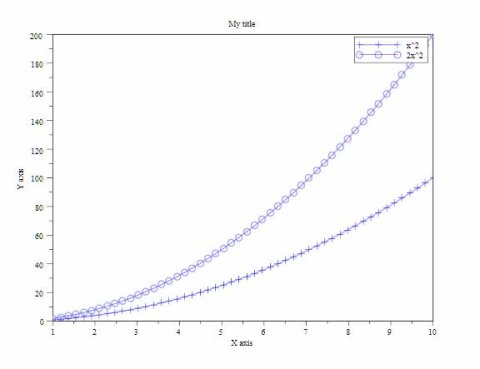
Figure 24: The x-y plot of a quadratic role – This is the same plot as in figure 21, with title and ten-y axes configured.

It may happen that nosotros want to compare two sets of data in the same 2d plot, that is, one set up of x data and two sets of y data. In the following script, we define the 2 functions f(x) = x^2 and f(10) = 2*x^two and plot the information on the same ten-y plot. Nosotros additionally use the "+-" and "o-" options of the plot function, then that we can distinguish the two curves f(ten) = x^2 and f(x) = 2*x^2.

function f = myquadratic ( x )
f = x^2
endfunction
function f = myquadratic2 ( x )
f = 2 * x^2
endfunction
xdata = linspace ( one , x , 50 );
ydata = myquadratic ( xdata );
plot ( xdata , ydata , "+-" )
ydata2 = myquadratic2 ( xdata );
plot ( xdata , ydata2 , "o-" )
xtitle ( "My title" , "Ten axis" , "Y axis" );
Moreover, we must configure a legend then that we tin know what curve is associated with f(ten) = x^2 and what curve is associated with f(ten) = 2*10^2. For this purpose, nosotros utilise the legend role in order to print the legend associated with each curve.

legend ( "x^two" , "2x^two" );
Effigy 25 presents the produced 10-y plot.

xyplot_legend

Figure 25: The x-y plot of ii quadratic functions – Nosotros have configured the fable so that we tin distinguish the 2 functions f(x) = x^2 and f(x) = two*x^2.

We now know how to create a graphics plot and how to configure information technology. If the plot is sufficiently interesting, information technology may be worth putting it into a report. To do so, we can export the plot into a file, which is the field of study of the side by side section.

three.5 Consign

In this section, we present ways of exporting plots into files, either interactively or automatically with Scilab functions.

Bitmap

Vectorial
xs2png	consign into PNG
xs2pdf	export into PDF
xs2svg	export into SVG
xs2eps	export into Encapsulated Postscript
xs2ps	consign into Postscript
xs2emf	export into EMF (only for Windows)
Bitmap
xs2fig	export into FIG
xs2gif	consign into GIF
xs2jpg	export into JPG
xs2bmp	export into BMP
xs2ppm	export into PPM

Figure 26: Export functions.

Nosotros can alternatively use the xs2* functions, presented in figure 26. All these functions are based on the same calling sequence:

xs2png ( window_number , filename )
where window_number is the number of the graphics window and filename is the name of the file to export. For instance, the post-obit session exports the plot which is in the graphics window number 0, which is the default graphics window, into the file foo.png.

xs2png ( 0 , "foo.png" )
If we want to produce higher quality documents, the vectorial formats are preferred. For example, LATEX documents may use Scilab plots exported into PDF files to improve their readability, whatsoever the size of the document.

ardwandrang.blogspot.com

Source: https://www.scilab.org/tutorials/getting-started/plotting

Share this post